Reinforcement Learning from scratch
Emmanuel Ameisen
22 Aug 2018
•
10 min read

Recently, I gave a talk at the O’Reilly AI conference in Beijing about some of the interesting lessons we’ve learned in the world of NLP. While there, I was lucky enough to attend a tutorial on Deep Reinforcement Learning (Deep RL) from scratch by Unity Technologies. I thought that the session, led by Arthur Juliani, was extremely informative and wanted to share some big takeaways below.
In our conversations with companies, we’ve seen a rise of interesting Deep RL applications, tools and results. In parallel, the inner workings and applications of Deep RL, such as AlphaGo pictured above, can often seem esoteric and hard to understand. In this post, I will give an overview of core aspects of the field that can be understood by anyone.
Many of the visuals are from the slides of the talk, and some are new. The explanations and opinions are mine. If anything is unclear, reach out to me here!
The rise of Deep Reinforcement Learning
Deep RL is a field that has seen vast amounts of research interest, including learning to play Atari games, beating pro players at Dota 2, and defeating Go champions. Contrary to many classical Deep Learning problems that often focus on perception (does this image contain a stop sign?), Deep RL adds the dimension of actions that influence the environment (what is the goal, and how do I get there?). In dialog systems for example, classical Deep Learning aims to learn the right response for a given query. On the other hand, Deep Reinforcement Learning focuses on the right sequences of sentences that will lead to a positive outcome, for example a happy customer.
This makes Deep RL particularly attractive for tasks that require planning and adaptation, such as manufacturing or self-driving. However, industry applications have trailed behind the rapidly advancing results coming out of the research community. A major reason is that Deep RL often requires an agent to experiment millions of times before learning anything useful. The best way to do this rapidly is by using a simulation environment. This tutorial will be using Unity to create environments to train agents in.
For this workshop led by Arthur Juliani and Leon Chen, their goal was to get every participants to successfully train multiple Deep RL algorithms in 4 hours. A tall order! Below, is a comprehensive overview of many of the main algorithms that power Deep RL today. For a more complete set of tutorials, Arthur Juliani wrote an 8-part series starting here.
From slot machines to video games, an overview of RL
Deep RL can be used to best the top human players at Go, but to understand how that’s done, you first need to understand a few simple concepts, starting with much easier problems.
1/It all starts with slot machines
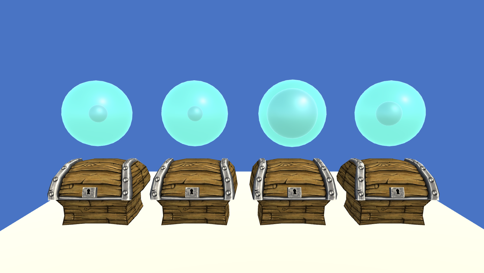
Let’s imagine you are faced with 4 chests that you can pick from at each turn. Each of them have a different average payout, and your goal is to maximize the total payout you receive after a fixed number of turns. This is a classic problem called Multi-armed bandits and is where we will start. The crux of the problem is to balance exploration, which helps us learn about which states are good, and exploitation, where we now use what we know to pick the best slot machine.
Here, we will utilize a value function that maps our actions to an estimated reward, called the Q function. First, we’ll initialize all Q values at equal values. Then, we’ll update the Q value of each action (picking each chest) based on how good the payout was after choosing this action. This allows us to learn a good value function. We will approximate our Q function using a neural network (starting with a very shallow one) that learns a probability distribution (by using a softmax) over the 4 potential chests.
While the value function tells us how good we estimate each action to be, the policy is the function that determines which actions we end up taking. Intuitively, we might want to use a policy that picks the action with the highest Q value. This performs poorly in practice, as our Q estimates will be very wrong at the start before we gather enough experience through trial and error. This is why we need to add a mechanism to our policy to encourage exploration. One way to do that is to use epsilon greedy, which consists of taking a random action with probability epsilon. We start with epsilon being close to 1, always choosing random actions, and lower epsilon as we go along and learn more about which chests are good. Eventually, we learn which chests are best.
In practice, we might want to take a more subtle approach than either taking the action we think is the best, or a random action. A popular method is Boltzmann Exploration, which adjust probabilities based on our current estimate of how good each chest is, adding in a randomness factor.
2/Adding different states
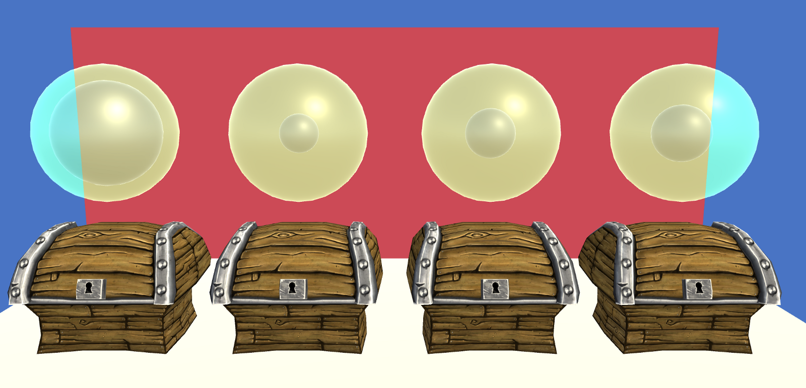
The previous example was a world in which we were always in the same state, waiting to pick from the same 4 chests in front of us. Most real-word problems consist of many different states. That is what we will add to our environment next. Now, the background behind chests alternates between 3 colors at each turn, changing the average values of the chests. This means we need to learn a Q function that depends not only on the action (the chest we pick), but the state (what the color of the background is). This version of the problem is called Contextual Multi-armed Bandits.
Surprisingly, we can use the same approach as before. The only thing we need to add is an extra dense layer to our neural network, that will take in as input a vector representing the current state of the world.
3/Learning about the consequences of our actions
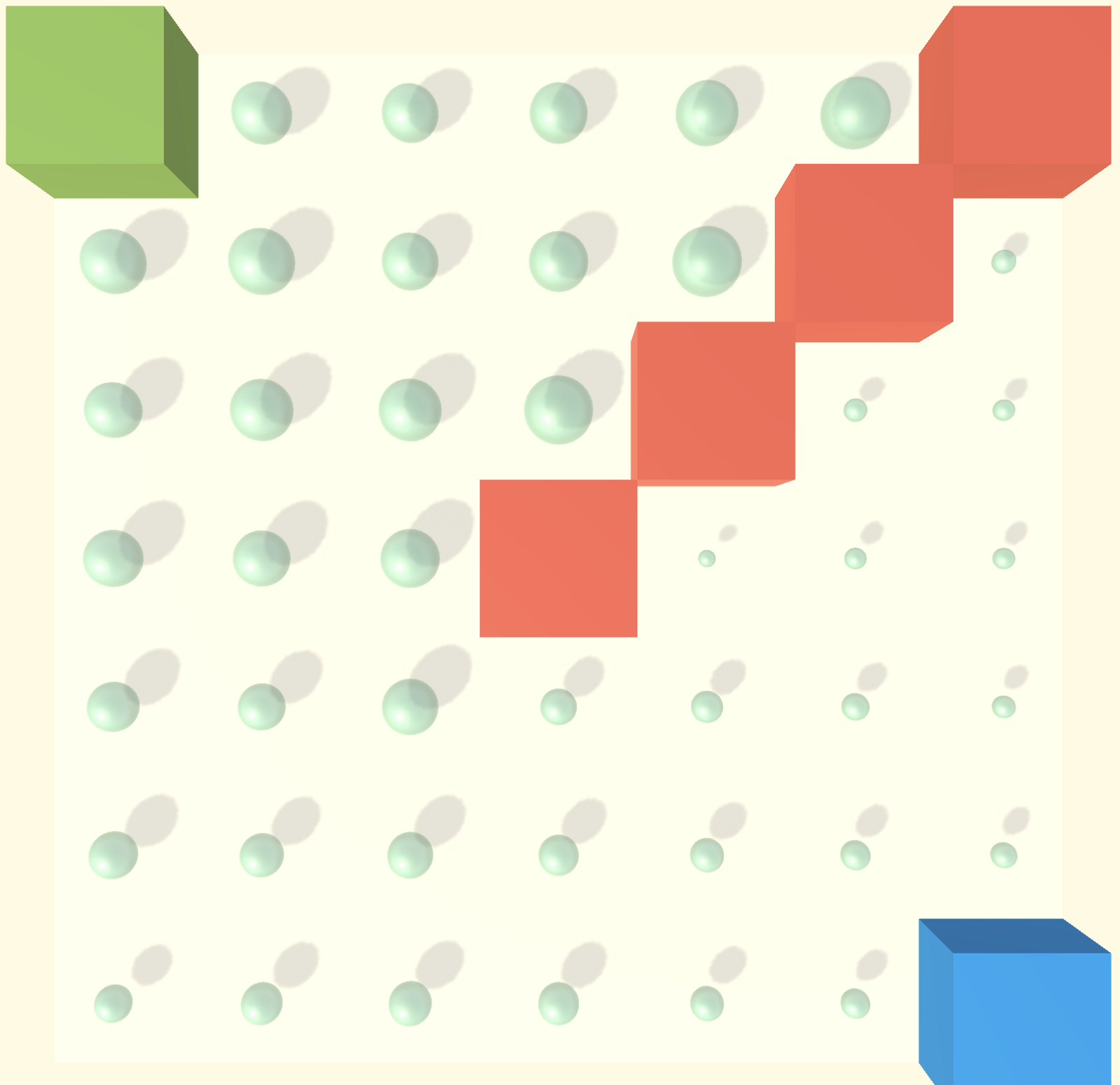
There is another key factor that makes our current problem simpler than mosts. In most environments, such as in the maze depicted above, the actions that we take have an impact on the state of the world. If we move up on this grid, we might receive a reward or we might receive nothing, but the next turn we will be in a different state. This is where we finally introduce a need for planning.
First, we will define our Q function as the immediate reward in our current state, plus the discounted reward we are expecting by taking all of our future actions. This solution works if our Q estimate of states is accurate, so how can we learn a good estimate?
We will use a method called Temporal Difference (TD) learning to learn a good Q function. The idea is to only look at a limited number of steps in the future. TD(1) for example, only uses the next 2 states to evaluate the reward.
Surprisingly, we can use TD(0), which looks at the current state, and our estimate of the reward the next turn, and get great results. The structure of the network is the same, but we need to go through one forward step before receiving the error. We then use this error to back propagate gradients, like in traditional Deep Learning, and update our value estimates.
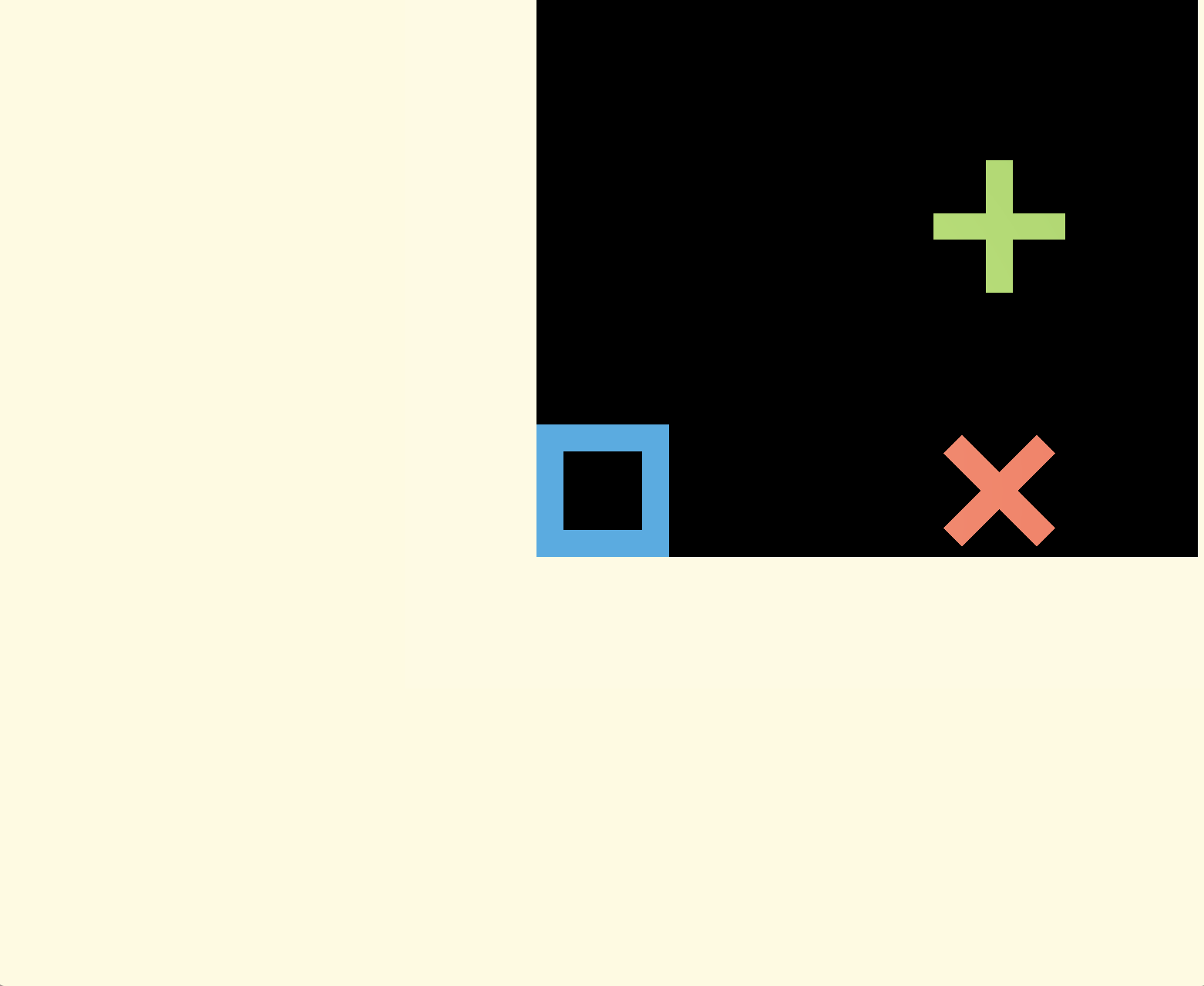
3+/Introducing Monte Carlo
Another method to estimate the eventual success of our actions is Monte Carlo Estimates. This consists of playing out the entire episode with our current policy until we reach an end (success by reaching a green block or failure by reaching a red block in the image above) and use that result to update our value estimates for each traversed state. This allows us to propagate values efficiently in one batch at the end of an episode, instead of every time we make a move. The cost is that we are introducing noise to our estimates, since we attribute very distant rewards to them.
4/The world is rarely discrete

The previous methods were using neural networks to approximate our value estimates by mapping from a discrete number of states and actions to a value. In the maze for example, there were 49 states (squares) and 4 actions (move in each adjacent direction). In this environment, we are trying to learn how to balance a ball on a 2 dimensional paddle, by deciding at each time step whether we want to tilt the paddle left or right. Here, the state space becomes continuous (the angle of the paddle, and the position of the ball). The good news is, we can still use Neural Networks to approximate this function!
A note about off-policy vs on-policy learning: The methods we used previously, are off-policy methods, meaning we can generate data with any strategy(using epsilon greedy for example) and learn from it. On-policy methods can only learn from actions that were taken following our policy (remember, a policy is the method we use to determine which actions to take). This constrains our learning process, as we have to have an exploration strategy that is built in to the policy itself, but allows us to tie results directly to our reasoning, and enables us to learn more efficiently.
The approach we will use here is called Policy Gradients, and is an on-policy method. Previously, we were first learning a value function Q for each action in each state and then building a policy on top. In Vanilla Policy Gradient, we still use Monte Carlo Estimates, but we learn our policy directly through a loss function that increases the probability of choosing rewarding actions. Since we are learning on policy, we cannot use methods such as epsilon greedy (which includes random choices), to get our agent to explore the environment. The way that we encourage exploration is by using a method called entropy regularization, which pushes our probability estimates to be wider, and thus will encourage us to make riskier choices to explore the space.
4+/Leveraging deep learning for representations
In practice, many state of the art RL methods require learning both a policy and value estimates. The way we do this with deep learning is by having both be two separate outputs of the same backbone neural network, which will make it easier for our neural network to learn good representations.
One method to do this is Advantage Actor Critic (A2C). We learn our policy directly with policy gradients (defined above), and learn a value function using something called Advantage. Instead of updating our value function based on rewards, we update it based on our advantage, which measures how much better or worse an action was than our previous value function estimated it to be. This helps make learning more stable compared to simple Q Learning and Vanilla Policy Gradients.
5/Learning directly from the screen
There is an additional advantage to using Deep Learning for these methods, which is that Deep Neural Networks excel at perceptive tasks. When a human plays a game, the information received is not a list of states, but an image (usually of a screen, or a board, or the surrounding environment).
Image-based Learning combines a Convolutional Neural Network (CNN) with RL. In this environment, we pass in a raw image instead of features, and add a 2 layer CNN to our architecture without changing anything else! We can even inspect activations to see what the network picks up on to determine value, and policy. In the example below, we can see that the network uses the current score and distant obstacles to estimate the value of the current state while focusing on nearby obstacles for determining actions. Neat!
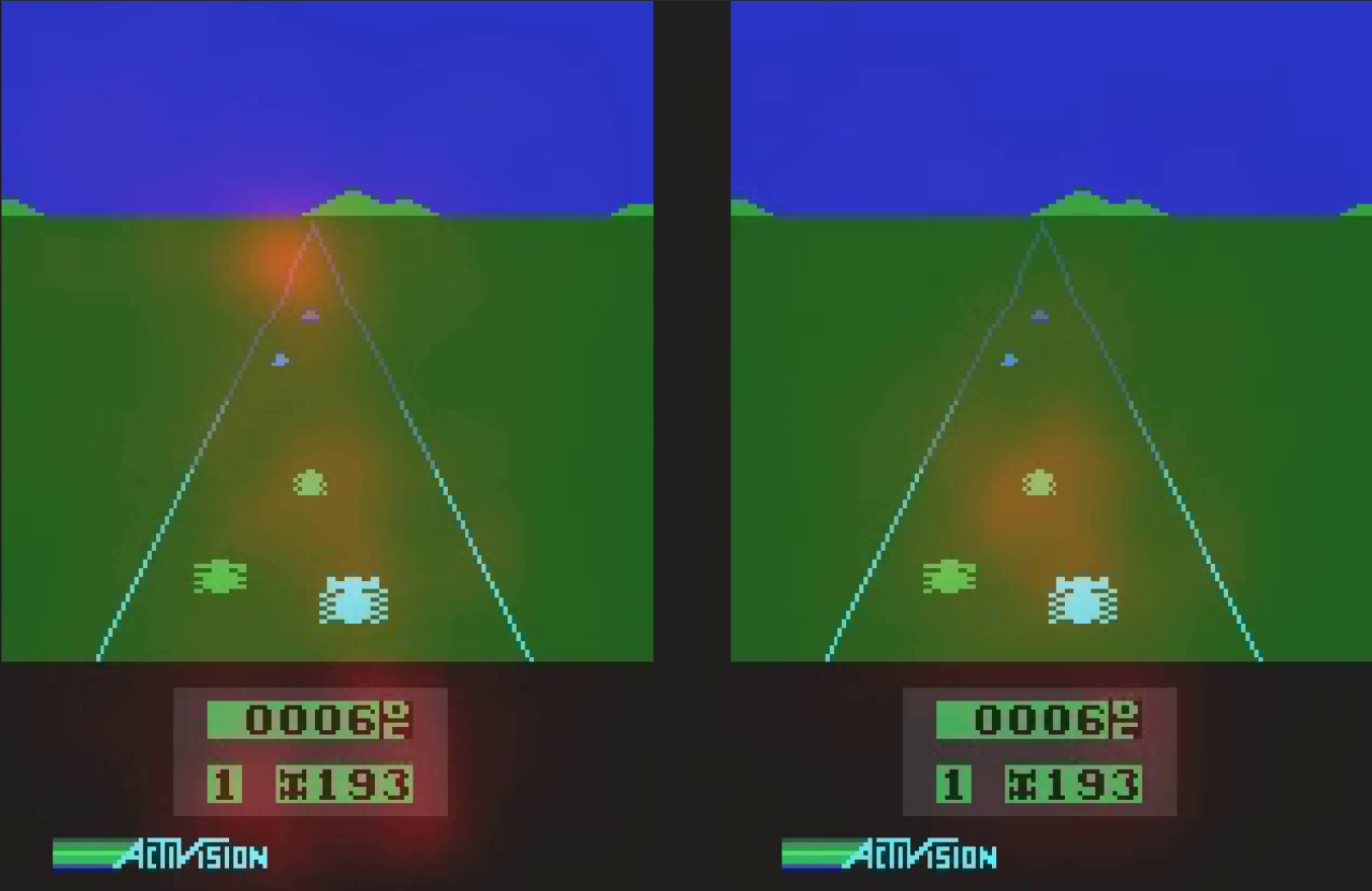
As a side note, while toying around with the provided implementation, I’ve found that visual learning is very sensitive to hyperparameters. Changing the discount rate slightly for example, completely prevented the neural network from learning even on a toy application. This is a widely known problem, but it is interesting to see it first hand.
6/Nuanced actions

So far, we’ve played with environments with continuous and discrete state spaces. However, every environment we studied had a discrete action space: we could move in one of four directions, or tilt the paddle to the left or right. Ideally, for applications such as self-driving cars, we would like to learn continuous actions, such as turning the steering wheel between 0 and 360 degrees. In this environment called 3D ball world, we can choose to tilt the paddle to any value on each of its axes. This gives us more control as to how we perform actions, but makes the action space much larger.
We can approach this by approximating our potential choices with Gaussian distributions. We learn a probability distribution over potential actions by learning the mean and variance of a Gaussian distribution, and our policy we sample from that distribution. Simple, in theory :).
7/Next steps for the brave
There are a few concepts that separate the algorithms described above from state of the art approaches. It’s interesting to see that conceptually, the best robotics and game-playing algorithms are not that far away from the ones we just explored:
- Parallelizing: A3C is one of the most common approaches out there. It adds an asynchronous step to actor critic, allowing the algorithm to run in a parallelized way. This allows it to solve more interesting problems in a reasonable amount of time. Evolutionary methods can be parallelized even more, and are showing very encouraging performance.
- Curriculum Learning: in many cases, it is extremely unlikely to get to any reward by acting randomly. This makes the exploration phase extremely tricky, as we will never learn anything valuable. In that case we can simplify the problem and solve a trivial version first, then use the basic model on increasingly more complex environments.
- Memory: Using LSTMs, for example, we can remember what happened in the past, and make decisions in a sequential way within a game playing session.
- Model based RL: Various approach exist for algorithms to build a model of the world while they learn, so that they can infer rules about how the world works, on top of simply performing actions with high rewards. AlphaZero combines an explicit model with planning. This is a paper I found particularly exciting in the space.
That’s it for this overview, I hope this has been informative and fun! If you are looking to dive deeper into the theory of RL, give Arthur’s posts a read, or diving deeper by following David Silver’s UCL course. If you are looking to learn more about the projects we do at Insight, or how we work with companies, please check us out below, or reach out to me here.
Thanks to Geneviève Smith, Ben Regner, Andy Mullenix, and Mari Kong.
WorksHub
Jobs
Locations
Articles
Ground Floor, Verse Building, 18 Brunswick Place, London, N1 6DZ
108 E 16th Street, New York, NY 10003
Subscribe to our newsletter
Join over 111,000 others and get access to exclusive content, job opportunities and more!